We use experiments to understand how to make new or better products or processes. Experiments cost time and money. However, by using some simple statistical tools to design and analyze our experiments, we can minimize the costs while maximizing the useful information we gain.

Before discussing designed experiments, we offer the following answers to the questions posed in the title:

What? Statistical design methods can help you determine the best combinations of variables to be used in an experiment. In statistically designed experiments, the design is coupled to the data analysis so that each complements the other to address the purpose of the experiment.

Why? Statistically designed experiments provide more information from fewer experiments than less sophisticated approaches. Furthermore, the conclusions and recommendations made based on the analysis of designed experiments are more rigorous and have greater validity than other design approaches.

When? Appropriate statistical design should be used whenever an experiment is conducted. Designs are available for comparative experiments, screening experiments, and optimization experiments. Each of these types of experimental designs are discussed in this article. 

In short, statistically designed experiments combined with the data analysis allow you to learn more and measure less.

Getting to a good design

This article presents a gentle introduction to the concepts of statistically designed experiments for different types of experiments. Since this is a gentle introduction, detailed design construction, the use of statistics, and data analysis are left for future articles.

Before addressing the nature of designed experiments, it is helpful to first discuss the nature of experimentation in general and what makes for a good experiment.

The first questions to ask are what is the difference between an experiment and a measurement and does it matter? Using the term experiment implies that the investigator is interested in how one or more variables (in statistics nomenclature the independent factors) affect one or more characteristics of something (the dependent factors or response factors). For example, we may wish to understand how independent factors such as the baking temperature and time affect response factors such as the color, texture, or other properties of a baked good. 

Measurement, on the other hand, implies that a characteristic is going to be quantified. For example, we can measure the temperature or the time or the color.  Measurement is the heart of process control and quality control. 

Thus, experimentation requires measurement but measurement does not require experimentation. It is the purposeful intent to study how the independent factors affect the dependent factors that distinguishes experimentation from measurement.

The experimentation process can be broken into six steps:

1. Specifying the purpose of the experiment;
2. Designing the experiment;
3. Conducting the experiment;
4. Analyzing and visualizing the data;
5. Conducting confirmation experiments (if necessary); and
6. Reporting the results, conclusions, and recommendations.

This article focuses on Steps 1, 2, and 4 of the experimentation process.

Specifying the purpose

When defining the purpose of an experiment, several questions should be addressed based on prior experience, expert knowledge, literature review, or other information sources:

• Why are you doing this experiment? What needs to be learned? These questions are vitally important and yet are often omitted or given cursory answers. An experiment intended to determine which independent factors actually have an effect on the response factor (as opposed to just believing that they might) is a very different experiment than one that is intended to optimize a production process, for example.
• What are your independent factors? What are the permissible ranges for them? Should some just be set at a fixed level and not studied?  Are there any combinations that won’t work or may present a safety hazard? The listing of the independent factors of interest is frequently one of the first questions answered. It is important to consider not only the obvious factors but also those that may be less apparent and have an impact. These factors should be included in the experimental design or controlled during the experiment so their impact is minimized.
• What are your dependent factors? How are they going to be measured? Are there critical or optimal values that should be targeted?  Identifying the response factors is usually a straightforward process. The technique to measure them has to have the required precision and accuracy to make the experiment worth doing.
• Do you have factors that may affect the response that can’t be controlled? How can their affects be minimized? Should they be measured and included in the data analysis? Not all factors can be controlled, but these nuisance factors may nonetheless affect the outcome of the experiment. For example, ambient conditions such as humidity may affect water sensitive products, so experiments conducted during a hot and humid summer afternoon may give different results than the same experiment conducted on a crisp and clear winter morning.
• How will you analyze the data? The specific nature of the analysis plays a critical role in determining the appropriate experimental design.  And, for many analyses, specific assumptions about the data are required.  Are those assumptions justified and, if not, what should be done about it?
• How many experiments can you do? Are there any restrictions on the order in which the experiments are done?  Will sufficient replicates be done to allow for a rigorous statistical analysis? These are often difficult questions to answer. The experimental designer will want to conduct as many experiments as possible to increase the reliability of the conclusions and recommendations. But the realities of cost, time, and other factors will limit the effort that can be expended, reducing the information that can be gained from the experiment.
• Are there any safety, environmental, or other hazards that must be considered? The question of safety should be addressed, both in design and conduct, to either mitigate the safety hazard or to avoid conditions that may present a safety hazard.

Factor scaling

Experimental design and data analysis are frequently done using scaled or coded units. This means that the independent factors have been scaled so they range from –1 to +1. For experimental designs, using scaled factors means generalized designs can be created that can then be used to determine the levels of the factors for a specific experiment. The analysis of experimental data using scaled factors removes any basis that may arise due to a difference in size or magnitude of the factors; it is more robust to analyze data where the factors are all of the same order of magnitude than widely different orders.

The traditional approach versus the design approach

The traditional approach to experimentation is often called the “one-factor-at-a-time” (OFAT) design. In an OFAT experiment, all but one of the factors are held constant while that one factor is changed in a systematic manner. Once one factor has been explored, it is held constant and another factor is varied. This process is continued until all the factors have been studied. 

Figure 1: Location of experiments for a one-factor-at-a-time experiment.

For example, consider an OFAT experiment examining just two factors. Suppose that one factor is held constant while the other is varied over five levels, after which the first factor is varied over five levels while the second factor is held constant. A graph of the factor levels for this experiment would look like Figure 1. This experiment fails to explore the extremes of the possible factor combinations and probably can’t be analyzed with sufficient accuracy to extrapolate the measured response into the corners of the space.

Designed experiments cover the entire experimental space. Using nine points in a designed experiment for two factors would fill the experimental space by conducting experiments at three levels of each factor. Now, since the experimental space is covered, the data can be analyzed to interpolate the results where the experiment was not covered.

The OFAT approach has several disadvantages:

• It provides less information about the experimental space for the same number of experiments,
• It provides less accurate estimates of how each factor effects the response,
• It does not provide an estimate of how the factors interact with each other to affect the

  Figure 2: Location of experiments for a simple designed experiment.

  response,
• It frequently is unable to identify the optimal settings of the independent factors, and
• It’s ability to estimate the response at points other than where the experiment was conducted is poor.

   

In short, the one-factor-at-a-time approach relies on doing an experiment at the “right” combinations of the factors, while the design of experiments approach relies on analyzing the data to find the “right” combinations.

Comparative experiments

Comparative experiments typically fall into two categories: (1) those where the response factors are measured and compared to standard values or (2) those in which two or more ostensibly similar items are measured and compared to each other. The classic quality control measurement is an example of the first case in which the question of whether the product meets the quality standards is answered. The second case is exemplified by questions such as whether the day on which something is produced affects the response.

Design

In general, the design of comparative experiments tends to be relatively straightforward. Since such experiments are intended to determine whether or not two quantities are the same, four outcomes are possible:

1. They are actually the same and the experimental conclusion is that they are the same;
2. They are actually different and the experimental conclusion is that they are different;
3. They are actually the same but the experimental conclusion is that they are different; or
4. They are actually different but the experimental conclusion is that they are the same.

From a statistical viewpoint, either of the first two outcomes is acceptable. The latter two, where essentially the wrong conclusion is reached, are known as false positives (type 1 or α errors) and false negatives (type 2 or β errors), respectively. To minimize the possibility of these errors, the primary design question is how many samples should be taken and analyzed. 

Data analysis

Figure 3: Mean location probability for three samples when sample 1 is not different from sample 2, sample 2 is not different from sample 3, but sample 1 is different from sample 3.

Data analysis for simple comparative experiments is perhaps some of the most common and easiest of statistical analyses to conduct. Analyses can be conducted to determine whether an average value is significantly different from a specified value or from another average. Similar comparisons can be made on the variation in the response quantified using the standard deviation.

When multiple means are to be compared, more advanced analysis techniques can be used.  Since these tests use the entire data set in the analysis, occasionally the results can be confusing. For example, a result such as “sample 1 is not statistically different from sample 2, sample 2 is not statistically different from sample 3, but sample 1 is statistically different from sample 3” would not be uncommon. Here saying “not statistically different from” is not the same as saying “is the same as” and so these tests, which take into the account the variability in the data used to determine the mean, can be subtler in their interpretation than other tests.

Data visualization

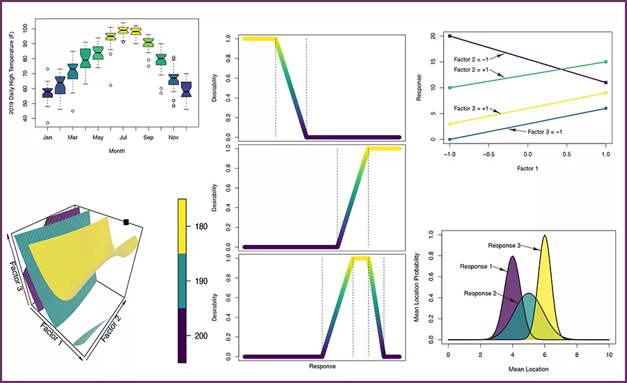
Convenient ways to visualize the results of comparative experiments are box-and-whisker plots. The box-and-whisker plot typically includes for each sample a box, a line or symbol near the middle of the box, the whiskers that extend outside the box, and symbols plotted beyond the whiskers.  Unfortunately, there is not an accepted consensus as to what each of these components means.  In the example figure, the bottom and top of the box represent approximately the first and third quartile of the data set, the bar in the middle of the box is the median of the data set, the whiskers are the median plus or minus 1.5 times the difference between the third and first quartiles, and the symbols represent “outliers” in the data.

Figure 4: Example box-and-whisker plot comparing average daily high temperatures.

Other possibilities in box-and-whisker plots are for the box bottom and top to be the mean minus or plus the standard deviation, the whiskers to be the 95% confidence interval around the mean, and the line in the middle of the box representing the mean instead of the median. Other statistical measures of the distribution can also be used. Because of this variation in what the elements of the plot mean, it is always necessary that they be explained in the description of the plot.

Screening experiments

Screening experiments are those in which the experimental question posed is something like: “Do any of these factors matter within the range over which they vary?” This type of question might be posed at the very beginning of developing a new production process or product. A second question, which can be asked at the same time if there are only a few factors or in a subsequent series of experiments if there are many factors, would be: “Do any of these factors interact with each other in the way in which they affect the outcome?”

The purpose of screening experiments, in statistical terminology, is to determine whether any main effects or interactions are different from zero.  A main effect is the difference in the average response at different levels of a factor. This is the same as asking whether or not the average response changed when the level of the factor changed.  A main effect can be determined for each factor. Two-factor interactions measure whether or not the magnitude of the change in the response when one factor was changed depends on the level of another factor. 

Design

Common designs for screening experiments are the factorial designs, the fractional factorial designs, and the Placket-Burman designs. For these designs each factor is studied at only two levels, the “low” and “high” levels designated in coded units by –1 and +1, respectively. Of these designs, the factorial designs require the greatest number of experiments and provide the most information; the Placket-Burman designs the fewest experiments and provide the least amount of information. The fractional factorials fall in between.  For most cases, factorial, fractional factorial, and Placket-Burman designs can be found in experimental design textbooks or using software packages.

The designs for the two-level complete factorial experiments are all possible combinations of the factors at their “low” and “high” levels. If N factors are being studied, a complete factorial requires 2^N experiments at a minimum since that does not include repetition of any of the experiments. The advantage of the complete factorials over the other screening designs is the ability to estimate interaction effects. A complete factorial can estimate not only main effects and two-factor interactions, it can estimate up to N-factor interactions. Other factorial designs use three levels of the factors or combinations of two and three levels.

Fractional factorials designs use a specified subset of the complete factorial designs. A half-fraction design requires ½*2^N = 2^N–1 experiments, a quarter fraction requires 2^N–2 experiments, and so on. Doing a subset of the complete factorial design does mean that some information that a complete factorial would provide is lost. However, when there are a large number of factors, some of which might not be statistically significant, these designs provide a method of estimating all the main effects and lower lever interactions using relatively few experiments.

The Placket-Burman designs are close relatives of the fractional factorial designs but are even more restrictive than the fractional factorial designs. They are capable under some circumstances of looking at more factors in fewer experiments than the fractional factorial designs.

Data analysis

Analysis of factorial, fractional factorial, and Placket-Burman designs to estimate main effects can be done using a variety of software packages or using a spreadsheet program. Analysis of variance (ANOVA) can be used to rigorously assess the presence and significance of main effects and interactions.  In the analysis of variance, the variation in the response values is separated into two components. One component is associated with changing the levels of the independent factors and one is associated with the natural experimental variability. By statistically comparing the change in the response due to the change in the factor level with the natural variability measured either through explicit or implicit experimental replication, conclusions can be drawn about the presence or not of main effects and interactions.

Data visualization

Figure 5: An interaction plot in which there is an interaction between factors 1 and 2 but not between factors 1 and 3.

In addition to box-and-whisker plots, interaction plots are also useful for screening experiments. To construct interaction plots, the factors are selected pairwise and one factor is plotted along the horizontal-axis and the average response at the high and low levels of the second factor are plotted. Responses at the same level of the second factor are then connected with straight lines. Since each factor is used at only two or three levels, the plots quickly and simply show both the main effects and two-factor interactions.

Optimization experiments

The objective of an optimization experiment is to create the equivalent of a contour or topographic map of the response as a function of the independent factors. This map is known as the response surface and it is used to estimate the settings of the independent factors that yield the optimum response. The map is created by using a polynomial equation fit to the experimental data using regression techniques to approximate the response throughout the experimental region.

Design

Experiments used to identify the parameter combinations that optimize the response of the system are some of the most challenging experiments to design. Whether the optimization is to minimize, maximize, or find the desired value of the response, the design depends on the shape of the experimental region, the anticipated complexity of the response surface, and the number of experiments to be conducted. Historical designs, such as the box-and-star designs and the Box-Behnken designs, were used when all the independent factors in scaled form could range from –1 to +1 with all combinations possible. Unfortunately, when the experimental space is restricted, these historical designs have been modified in ways that do not always produce high-quality designs.

Recently, the I-optimal criterion has been used to create satisfactory designs. The I-optimal criterion minimizes the average prediction variance over the experimental space. Application of the I-optimal criteria results in designs that give the best prediction values possible.

Data analysis

Figure 6: Prediction variance heatmaps for a poorly designed (top) and locally I-optimal designed (bottom) experimental plan for a constrained 2D space. In these plots, darker contours represent smaller values of the prediction variance.

For optimization experiments, the basis of the data analysis is to use regression techniques to fit a model equation to the experimental data and then use this model to identify the parameter combinations that optimize the response. This does not require that those specific combinations were used experimentally; in fact, the model is used to interpolate between the experimental conditions.  Once the optimal combinations have been determined, additional experiments are done at those conditions to confirm the predicted response. For this approach to be simple but successful, the initial response surface model is usually either a complete quadratic or cubic polynomial. This selection should be made prior to the design of the experiment so the necessary levels of the factors can be included in the design.

For optimization experiments the data analysis should have several steps to ensure the validity of any conclusions. These steps should include:

1. A preliminary visual data review to ensure that there is nothing completely unexpected and no gross errors were made,
2. Selection and verification of the appropriate model to ensure that it adequately represents the experimental data and that the assumptions made in creating the model are valid,
3. Model application where the optimum conditions are estimated (usually numerically), and
4. Confirmatory experiments at the optimum conditions to ensure that the predicted responses are realized.

Because of the magnitude of the undertaking, several separate analyses are conducted during an optimization experiment. These include:

Figure 7: Desirability functions for “less than,” “greater than,” and “between” criteria.

• Model reduction to eliminate terms from the initial model that are statistically not significant to prevent over-fitting the data,
• Verification of the assumptions that the residuals (the difference between the experimental values and the values predicted using the reduced model) are randomly and normally distributed,
• Identification of any outliers or influence points in the data set,
• An analysis of variance to verify there is not a statistically significant lack-of-fit between the reduced model and the experimental data,
• Model application, and
• Estimation of the uncertainty in the model predictions.

When optimizing multiple responses, it is highly unlikely that the optimum factor combination for all the responses will be the same. To overcome this, desirability functions are written for each response, the overall desirability is constructed from these individual functions, and the overall desirability is maximized. The three most used desirability functions are for a desired response less than a given value, greater than a given value, or between two given values.  When a criterion is met, the desirability function has a value of 1.  When it is “almost” satisfied, it ranges from 0 to 1.  When it is “not” satisfied, it has a value of zero.  The overall desirability is then determined as the product of the individual desirability values.

Data visualization

Figure 8: Iso-surfaces at constant values of the predicted response and the predicted minimum in the experimental space.

Several different data visualization tools are used in the analysis of an optimization experiment.  The preliminary data review can simply be plots of the response, on the y-axis, versus an independent factor on the x-axis. Other plots and analyses can be used to verify the model assumptions and to detect points that may have an overly strong influence in the model predictions.

Of course, the most needed visualization is that of the final model.  When there are only two independent factors, simple contour plots can be used. For three-factor optimization problems, surfaces at a constant value of the response (iso-surfaces) can be drawn to help elucidate the shape of the response surface.

Summary

Designed experiments paired with statistical analysis of the data should be used for a wide range of experimental conditions. Designs which minimize the number of experiments while maximizing the information obtained can be created for comparative, screening, and optimization experiments. This gentle introduction has not tried to provide a complete discussion about the designs nor the data analysis. Instead, it has attempted to provide guidance as to what, why, and when designed experiments should be used.

For more information, contact Stuart Munson-McGee via email: sh.munsonmcgee@gmail.com